Practical Implementation of PCA
The first time I encountered PCA(Principal Component Analysis) as a concept was in a Thinkful’s Introduction to Data Science Course. As much as
I can remember I was baffled and bewildered. For weeks I couldn’t make
head or tail of what it means and the ‘job’ it is meant to do in machine learning and data science. However, a considerable milestone was attained when my mentor concurred with my suggestion that it is similar to the Pareto Principle or the law of the vital few. The law of the vital few states that ‘for many outcomes, roughly 80% of consequences come from 20% of the causes’. In other words, 80% of the components of a subject lies in 20% of such components.
When ‘PP’ is juxtaposed with Principal Component Analysis, the problem is then reframed as “how to reduce the component that makes up a subject to as few components as possible without losing the meaning of such a subject”. Thus Principal Component Analysis from the perspective of machine learning and Data Science is a complexity-reduction technique that tries to reduce a set of variables down to a smaller set of components that represent most of the information in the variables. Through this transformation, a large chunk of the information across the full dataset is effectively compressed in fewer feature columns. It is the most popular Dimensionality Reduction Algorithm used in various operations like:
- Noise Filtering
- Feature extraction
- visualization
- Gene Data analysis
- Stock market prediction e.t.c
Keeping with the spirit of this blog, I shall not bore you with unnecessary mathematical theories/jargon about PCA; we shall concentrate on how I often apply it in model building exercise. However, you can read more about the mathematical foundation of PCA. There is A Tutorial on Principal Component Analysis by Jonathan Shlens at the Salk Institute.
To this end, in this post, I shall cover PCA in the following sub-categories/steps:
- Initialization, Standardization & Transformation
- Explained Component Summary Report
- Decision: How many components?
For effective coverage we shall demonstrate with simple dataset
Initialization & Standardization & Transformation
 #import necessary package and Modules
 import pandas as pd
 import numpy as np
 import seaborn as sns
 import matplotlib.pyplot as plt
 from sklearn.preprocessing import StandardScaler
 from sklearn.decomposition import PCA
To perform a PCA operation effectively the dataset must be Standardized and an object must be created from the PCA class
#read data unto pandas
mydata = pd.read_csv('https://raw.githubusercontent.com/Thinkful-Ed/data-201-resources/master/ESS_practice_data/ESSdata_Thinkful.csv')
mydata.head()

For brevity we shall select four features only which is more than enough to demonstrate.
mydata.columns

mydata[['tvtot', 'ppltrst','pplfair','pplhlp']]
mydata.head()

#Standardized data and place result into a pandas DataFrame
mydata_std = pd.DataFrame(StandardScaler().fit_transform(mydata), columns= mydata.columns)

#initte PCA
pca = PCA(n_components=4)

#get pcs version of data
mydata_pca = pd.DataFrame(pca.fit_transform(mydata_std), columns=mydata.columns)
mydata_std.head()
mydata_pca.head()


Explained Component Summary Report
As a convention, normally I produce a report which makes the PCA operations easy to digest. And we do this with the three methods:
- explained variance: These are the variance components accounted for by each principal component, in descending order. The sum of these variance components is the total variance.
- explained variance ratio: These are the proportion of total data variance accounted for by each principal component, in descending order. They sum to
1.0 - Singular values: These are used to calculate the variance components.
pca.explained_variance_
pca.explained_variance_ratio_
pca.singular_values_

# summary Report
data = { 'Singular Value':pca.singular_values_,
         'Variance':pca.explained_variance_,
         '%Variance':pca.explained_variance_ratio_*100 }
var_report = pd.DataFrame( data )
var_report[ 'Cum Sum' ] = var_report[ '%Variance' ].cumsum()
print( 'Number of observations: n = {}'.format( pca.n_samples_ ) )
var_report

The Variance is the contribution to the total variance of the data and is based on the singular values. Thus the sum of the Variance contribution is the total variance. The first principal component accounts for 51.5% of the variance and the first two account for 75.8%.
Decision: How many components?
The biggest decision to make when running a PCA is how many components to keep. There are several rules to guide us in choosing the number of the component to keep. The most straightforward is to keep components with eigenvalues or where Singular value is greater than 1 as these components add value. (because they contain more information than a single variable)
Another rule is variance cutoffs where we only keep components that explained at least x% of the variance in the data.
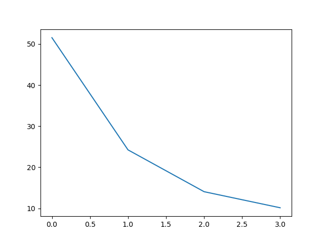
Yet another rule is to visualize the eigenvalues in order from highest to lowest connecting them with a line. This is also called the scree plot.
#plot scree plot
plt.plot(var_report['pctVariance'])

From visual inspection, we shall keep all the component whose eigenvalues or pctVariance values falls above the point where the slope of the line changes the most drastically.This is also called the ‘elbow’ point.Thus 24% and above will form our components.
In the course of this practical post, we have come to understand the significance of PCA operation in the machine learning process. We also demonstrate the simplest and effective way of analyzing the PCA decision process, which, actually is the most important step, as the primary purpose for undertaking a PCA operation invariably is to reduce features!
I hope you have learned something today. Bye!